Remote Observing at the Lowell Discovery Telescope

Overview

    This last week, as part of my astronomical observing class (ASTR4880: Astrophysical Measurements) at UToledo, I helped observe remotely at the Lowell Discovery Telescope in Arizona on October 25th, 2023.

    This post goes through the observing and data-reduction process.

Observing

Preparation

    In preparation for this observing opportunity, each of us picked our source. These were chosen primarily from the list of Messier objects, with some filtering due to position and brightness.

    As part of this, I produced airmass charts for a set of sources with sensible right-ascension and declination, then picked one that I believed would be both particularly bright, and would look pretty in a final image.

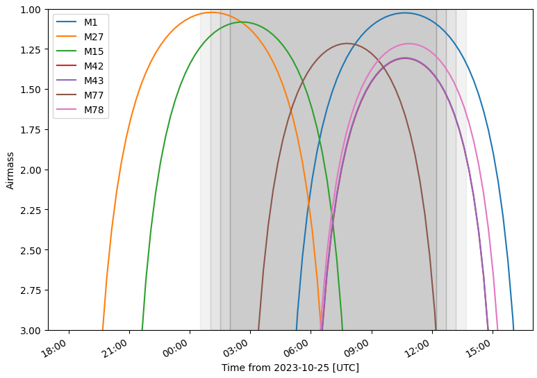Airmass chart of several candidate objects for observation.

    The object that I chose ended up being M27, a planetary nebula that would be above 1.5 airmass for the first few hours of astronomical night. I was then able to create a finder chart for this object, as well as identify the time-range that M27 was above 1.5 airmass.

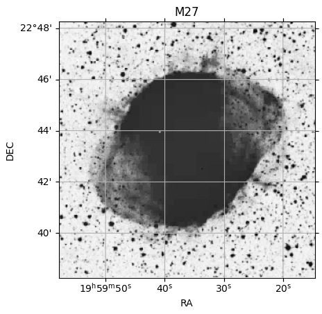A finder chart for M27

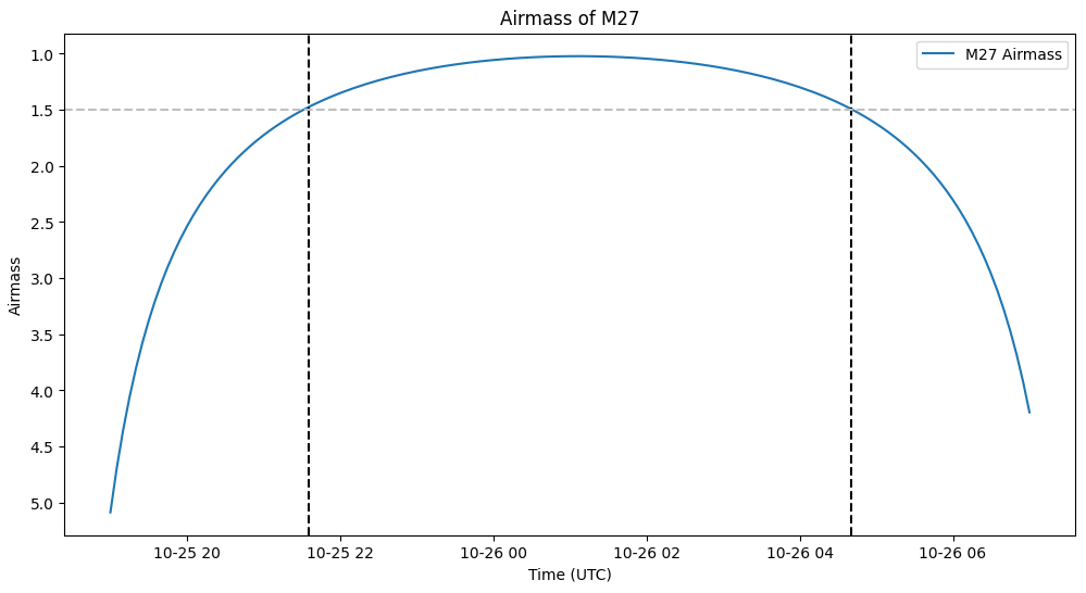An airmass chart for M27

    My object was then added to a spreadsheet containing the other students’ sources, with a section for desired filters. I chose V, B, and H-alpha as my filters, as I thought that, in addition to the V and B, the H-alpha would help track some of the geometry that the V and B wouldn’t catch.

Observing

    Dr. Smith and a few of my classmates were there in person, while the rest of us were remoting in from the remote observing room at the Ritter Astrophysical Research Center. I arrived at the remote observing room at about 8:00pm, and we stayed in that room until about 3:00am.

    The remote observing room is equipped with several TV screens and a conference video camera, using which we started a zoom call with the people at the LDT that allowed us to communicate back and forth.

    Much of the beginning of the night was spent taking a tour of the LDT, with the remote version provided by Dr. Smith’s smartphone. Once the director had left, the telescope operator helped us set up the telescope operating software, which prepared us for our night of observing.

    I spent the majority of my time keeping the observing log updated, which included things like the output filename, the filter and exposure time used, the starting time, and the current airmass, seeing, and target. Much of this information was likely superfluous, however it will likely prove to be useful experience for future observing experiences.

Results

    Our night was relatively successful; we were able to take the requisite bias-frames and dome-flats in the 5 filters we planned on using, and we were able to take exposures in three filters for one of our sources (IC5146). Unfortunately, due to cloudy weather, climbing humidity, and smoke concerns early in the night, we were only able to take about 30 minutes of exposures.

    We spent quite some time taking the dome-flats, much of which was spent experimenting to find an exposure time that would yield decent results, which we defined as an average value of ~20,000 in the pixels. We took 4 flat exposures for most of the images, with the exception of H-alpha(on), which only recieved 2 usable flat exposures due to lamp issues on the dome screen, as well as OIII and U, which only recieved two and one exposure, respectively, due to their rapidly ballooning exposure times.

    It was at around this time that we had a brief, 30 minute window when the smoke had died down and the humidity was still low enough for us to observe. We took this opportunity to get as many exposures as we could, and as such we focused on the filters with the lowest expected exposure times in order to maximize the number of exposures we could get.

    We focused on the very bright IC5146 source, in part because it was the brightest target with the lowest airmass during our window from our list of prepared targets. We ended up with exposures in the V, B, and H-alpha(on) filters, with 4, 4, and 2 exposures respectively.

    Following this, while we waited for the humidity to decrease, we took the bias-frames for the telescope, with a resulting 19 exposures.

    After some more time spent waiting, we decided to call it quits, as the humidity was predicted to keep increasing, and the predicted cloud cover had rolled in. There had also been a target-of-opportunity scheduled for early in the morning on our observing time, however due to the cloud cover and conditions, the researcher was contacted and canceled their observing request. As such, we were able to leave early at about 3:00am, rather than staying there all night.

Data Reduction

    After a several-day break to work on other projects and schoolwork, I spent some time sunday night and monday morning working on reducing the data, and was able to put together a preliminary 3-color image before class on monday.

Creating Biases

    Using the bias frames we took, I was able to layer the bias exposures and take the median value, creating a ‘super-bias’ that can be used to help reduce the impact of the dark-current from the CCD on our final images.

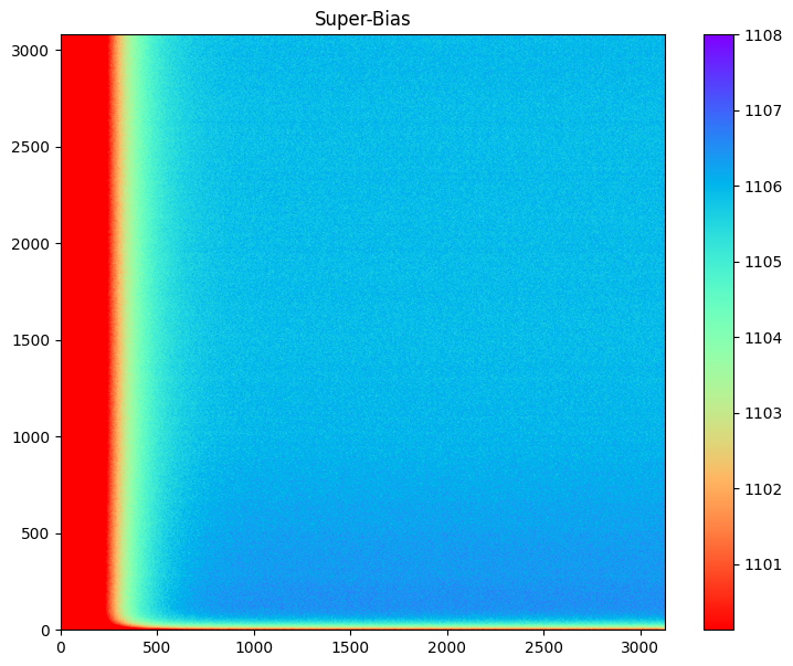A combined bias for the Lowell Discovery Telescope

Creating Flats

    Using the dome-flat exposures, I was able to create a ‘super-flat’ for each of the bands, which can be used to reduce the impact of differences between each pixel’s response, as well as the impact of dust grains on the filters.

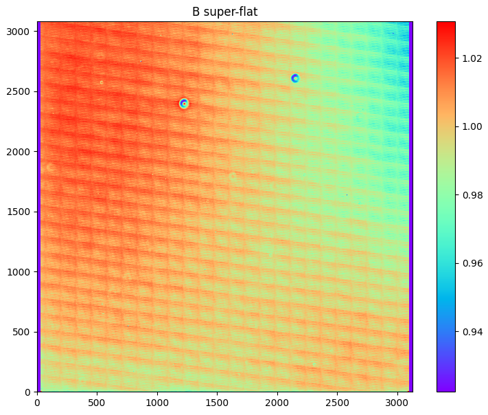A combined Flat frame for the B-band of the Lowell Discovery Telescope

Creating Reduced Images

Theoretical Basis

    For each of the remaining science images, we can use the following formula to incorporate our ‘super-bias’ and ‘super-flat’ images to produce better images.

\[I_r = \frac{I - B}{F*t}\]

Where;

• $I_r:$ reduced image

• $I :$ original image

• $B :$ ‘super-bias’ image

• $F :$ ‘super-flats’ image

• $t : $ exposure time

    By subtracting out the bias frame from the original image, we can remove much of the ‘dark current’, or the values that the CCD returns even when there is no light hitting the detector.

    By dividing by the flat times the exposure time, we can account for the effect of the filter on the light at each moment, where areas that are higher in the Flat image received more light through the filter than the places that are lower.

    The final result of this is our reduced image, which is much cleaner than our initial image, and is much less affected by certain sources of instrumental error.

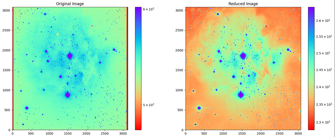A comparison showing an original image, and the reduced image for one exposure in the V band

Initial Results

Preliminary Three-Color Image

With the images reduced, I decided to quickly throw together a three - color image before class on monday. Using some matplotlib LogNorm objects and matplotlib’s imshow function, I was able to produce the following three color image;

An early 3-color image I produced using python

Issues

    It wasn’t until I discussed my results with the professor that a major issue came to light; I had assumed that each image was perfectly aligned, which was not the case. In reality, the tracking on the LDT, while excellent, isn’t perfect, and the resulting images are shifted slightly from each other. the three color image does show this somewhat, especially in the smaller point sources in the background.

Resolving Tracking Issues

        In order to fix this shifting, I was recommended the package astroalign, which would allow us to, given a target image, shift a different image to match position with that target image. I selected the V band as the target image, as it seemed the clearest of the three. After some tuning for the H-alpha image, I was able to match the three images together, correcting for the slight shifting.

Final Results

Three Color Image (Python)

Basic RGB

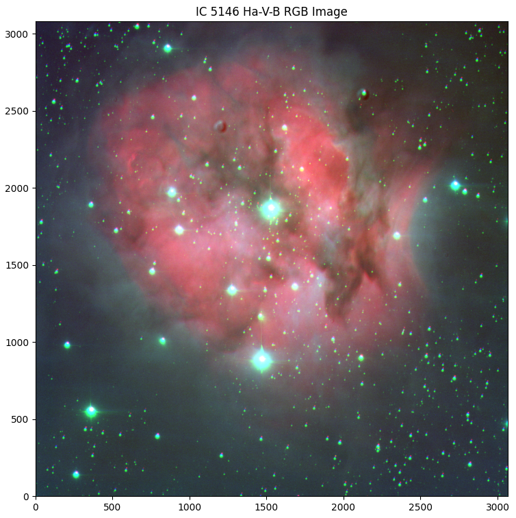
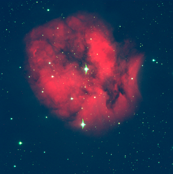
    Using the same process as before, but this time with the images corrected for shifting, I was able to create a much cooler looking three color image.

A final, aligned 3-color image of IC5146.

Adding WCS with astrometry.net

As a result of our processing steps, the WCS that was present on our image initially had been mangled, and our resulting image no longer has this useful information. There exists a very convenient solution to this problem, specifically the website astrometry.net. This website can take an uploaded fits image and automatically determine and apply the proper coordinates to the fits file, which can then be downloaded. The one thing to note is that these images are uploaded and made available publicly, so this method should only be leveraged in cases where that kind of public available isn’t a problem.

Three Color Image (DS9)

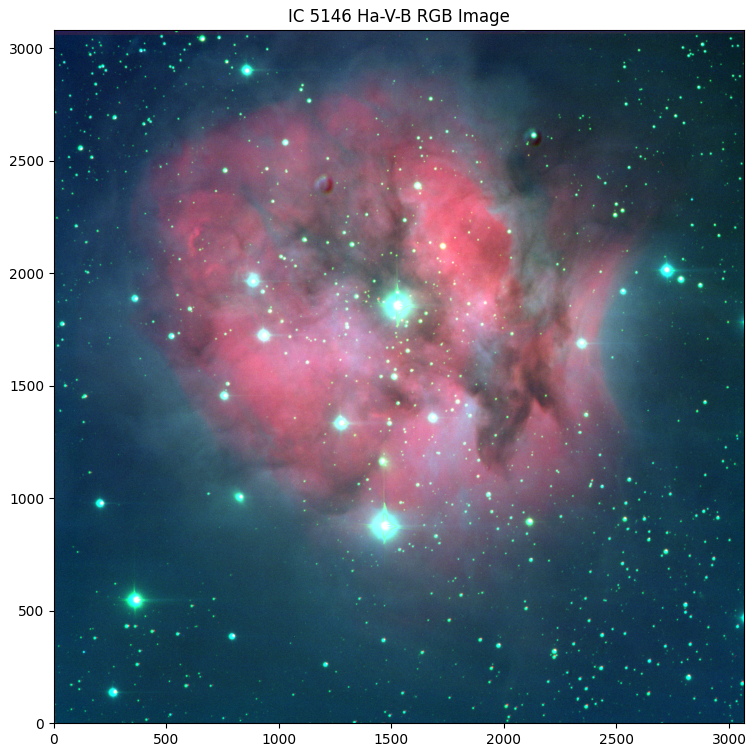
    I also spent some time creating a three color image in DS9; the benefit to this approach is that it allows more immediate control over the brightness and contrast of each individual filter. After some work, I was able to make an image that I was happy with;

A 3-color image of IC5146 produced using DS9 software.

Final Thoughts

    Overall, my first experience in observing was, in my opinion, a success. While we didn’t really get to observe much more than a single source, we were still able to observe in some capacity, as well as create the necessary calibration images.

    This process also gave me an opportunity to practice the process of image reduction, and the different ways to create 3 color images from a set of files.