Research Update - Week 13
This week’s post will be fairly short, as I spent most of my time this week finalizing some of my upcoming graduate school applications, and I took advantage of thanksgiving break to do so.
Cosmology Group
Changes to Model
One thing that I have been working on this week has been trying a few ideas I had for ways to improve the operation of the model. These were focused on trying to implement the density field, as we believe that to be the main way we will better replicate the renaissance results.
Change to Bubble Centering
My first step was to investigate a small simplification that I had devised. The original model placed ionized regions in a two step process; First, it convolves through the box and identifies the centers of bubbles, then convolves a second time to turn these bubble centers into full bubbles. This process is done individually for a set of 30 logarithmically spaced bubble scales.
One issue that had been addressed in the original model was a consistent overshooting effect. Due to the way that bubble centers were placed, the
Change to Density Consideration
The main method that caught on, however, was a set of changes that involved the density field, and were wildly effective at replicating the renaissance results.
My change was somewhat fundamental, and dealt with how the model determined the density of a location. Originally, the model would take the average density over a region, compare it against the average photons for that region, and place a bubble center if that location was ionized. Instead, my method only considered the density of that specific pixel against the average photons, rather than the average density.
My logic for this change was that, rather than considering the bubble centers, I would instead consider the ionization at each pixel. The averaging at different scales would represent the distribution of photons at different levels of spread out, with the assumption that the photons would distribute evenly throughout a spherical bubble region at a uniform density. This meant that, for each pixel, we would find how many photons would have ended up at that location for this level of ‘spread out’, which could be compared against the gas density in order to determine ionization.
This approach mitigates the largest problem with including the density field, where our assumption of perfectly spherical bubbles conflicts with reality, where bubbles push through dense filaments before ionizing their surroundings. This means that, unlike in reality, our model would attempt to ionize the dense filamentary region immediately surrounding the halo, which would suppress all but the very largest bubbles from forming.
In contrast, this method produced genuinely surprising results. There are still issues, which I will enumerate on shortly, but the current output is already outperforming the existing models on many of the metrics of success we have been describing. I will also note that this model has not been tuned for ionization fraction yet, and is currently about 1/4th the ionization fraction of the renaissance model.
Firstly, and likely of the most interest, the starless halo ionization plots show that this new variation is a vast improvement over the existing models, with the output actually reasonably matching the renaissance curve.
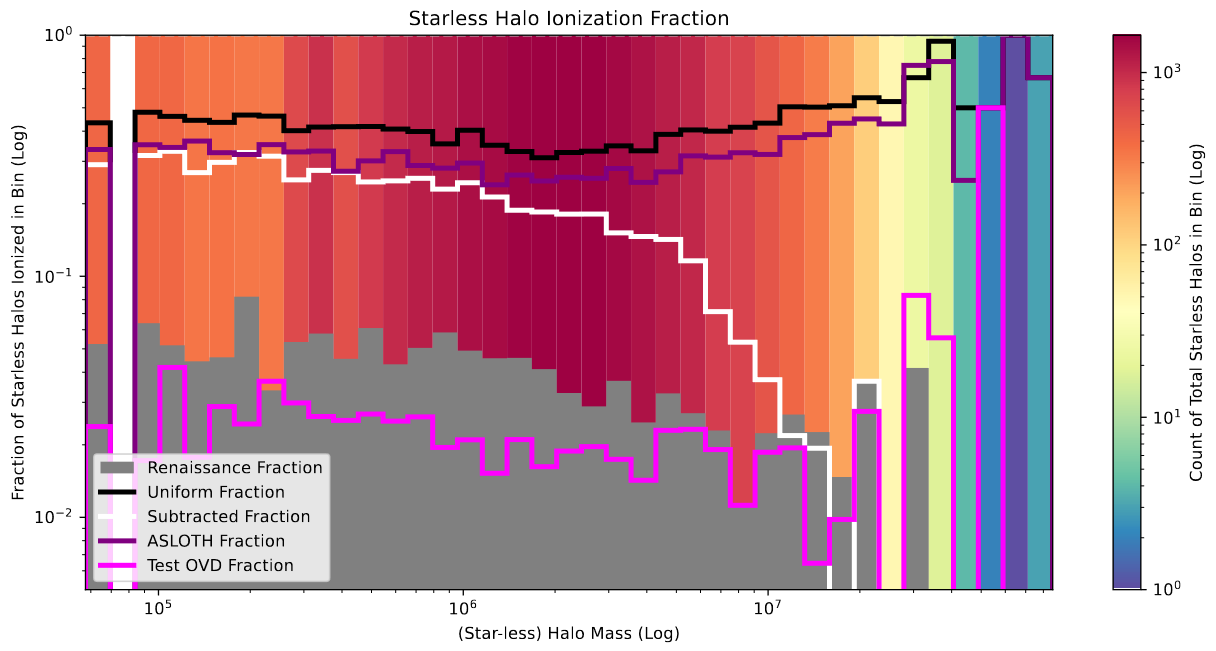 Starless Halo Ionization plot showing the much better agreement with the model variant
Next, the bubble volume distribution plots are somewhat less positive, with the distribution being much more skewed towards the low end, with many more single pixel bubbles in this new density field than in the renaissance ionization, and the overall result matching less perfectly than the uniform model does. The overabundance of smaller bubbles is likely due to an issue that I will discuss in more detail below.
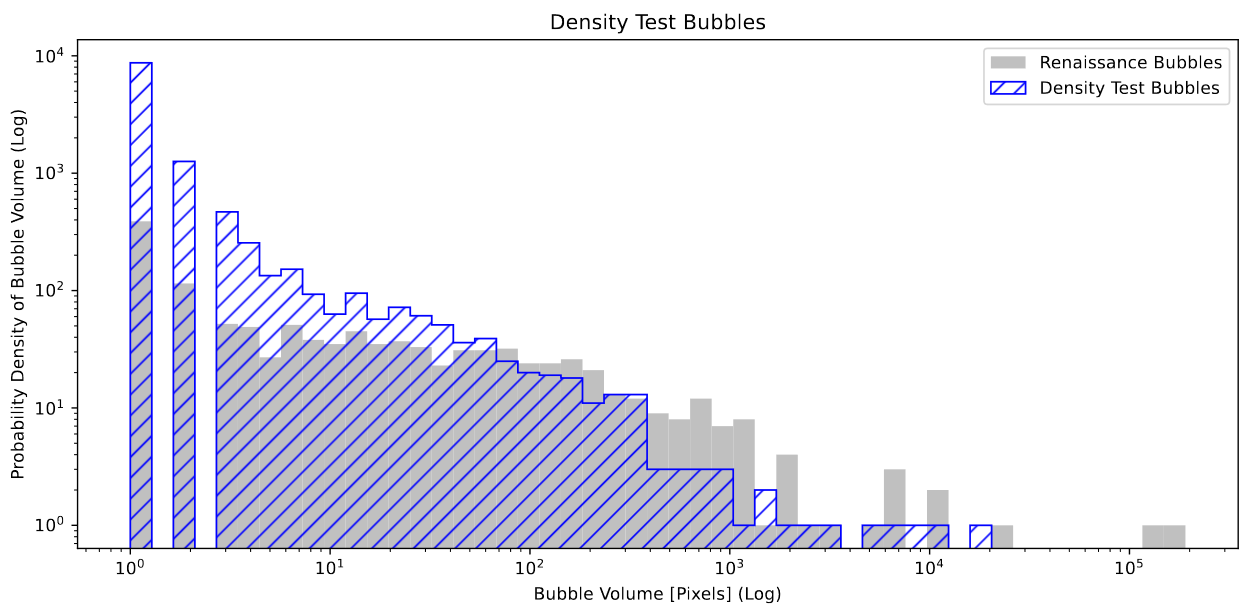 Bubble Volume plot comparing renaissance and the new model variant
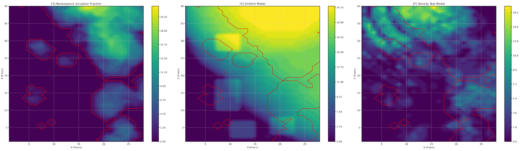
One other plot to examine is the halo slice plots, which seemed to show that the new variation would perform either equally or better when compared to the existing model, with the main disagreement coming in areas of renaissance that are known to possess complexities that our current model lacks the information to replicate. There is also further strange geometry that can be better explained by the issue that I will enumerate on below.
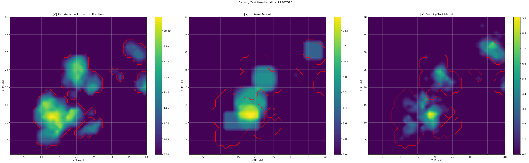 halo slice plot comparing the output of this model variant with the renaissance output and uniform model.
The issue I mentioned previously is one of geometry. When examined visually, there exists a pattern of ‘shells’ to many of the bubbles in this new model, where instead of a single solid structure, the bubble is comprised of several layers of hemi-spherical shells, as shown below.
 halo slice plot comparing the output of this model variant with the renaissance output and uniform model. This case is important specifically because it demonstrates the odd layering effect.
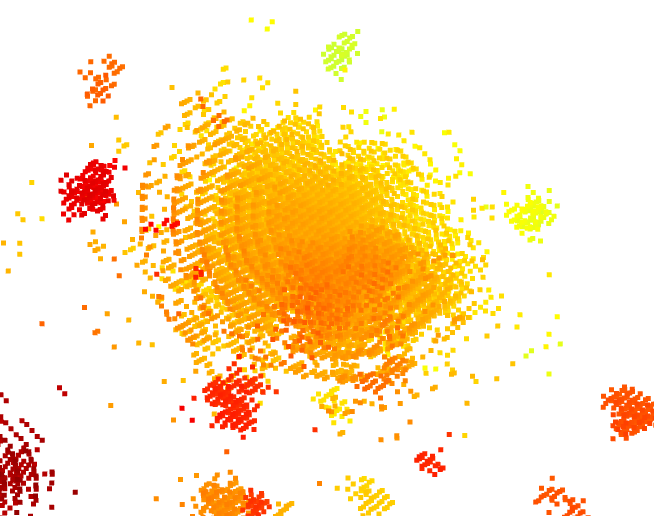 image of a portion of the model output that shows this shell behavior.
My initial theory was that this was related to the different bubble scales that the smoothing was done over, which was proven correct when I doubled the scale resolution from 30 to 60, and the presence of these shells was diminished, but not removed entirely.
More Methods for Comparing Output
I also spent some time this week working on a few additional methods for characterizing the output of the models, and comparing their effectiveness.
One of the more effective results was one that compares the ionization fraction between a model and renaissance. Rather than comparing over the whole box, this method randomly samples several hundred thousand smaller boxes (of a specified size) at the same locations between the two boxes, then compares the results as a 2-dimensional histogram. One result is shown below, for the uniform model.
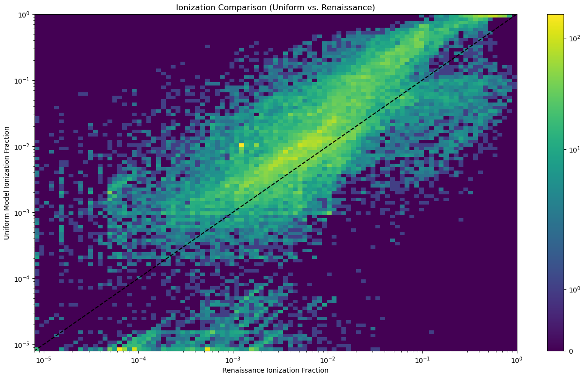 ionization comparison plot, comparing renaissance and the uniform model through small box samples.
This plot turned out to be somewhat effective, in that it seems to mimic some of the effects we had observed. Specifically, we see that, at the more ionized regions in renaissance, the uniform model consistently overshoots the size of these bubbles, which is reflected in this graph by the points moving above the agreement line, and indicating that the uniform model was significantly more ionized than the renaissance values at these locations.
A different avenue that I explored was attempting to determine, for each halo, the distance to the nearest ionized region, as well as the distance to the nearest neutral region. I did this by first isolating the edge pixels of each ionized region (using some code I had written several months ago), then used open3D to establish these pixels as points within a point cloud, then used the provided functions to determine the distance to the closest edge pixel from each halo, which indicated both the distance to the nearest ionized region for neutral halos, as well as the distance to the nearest edge of the bubble for the ionized halos.
I was then able to plot a distribution for both cases, with the following results;
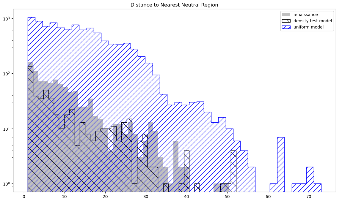 histogram showing the distribution of the distances to the nearest neutral region for ionized halos.
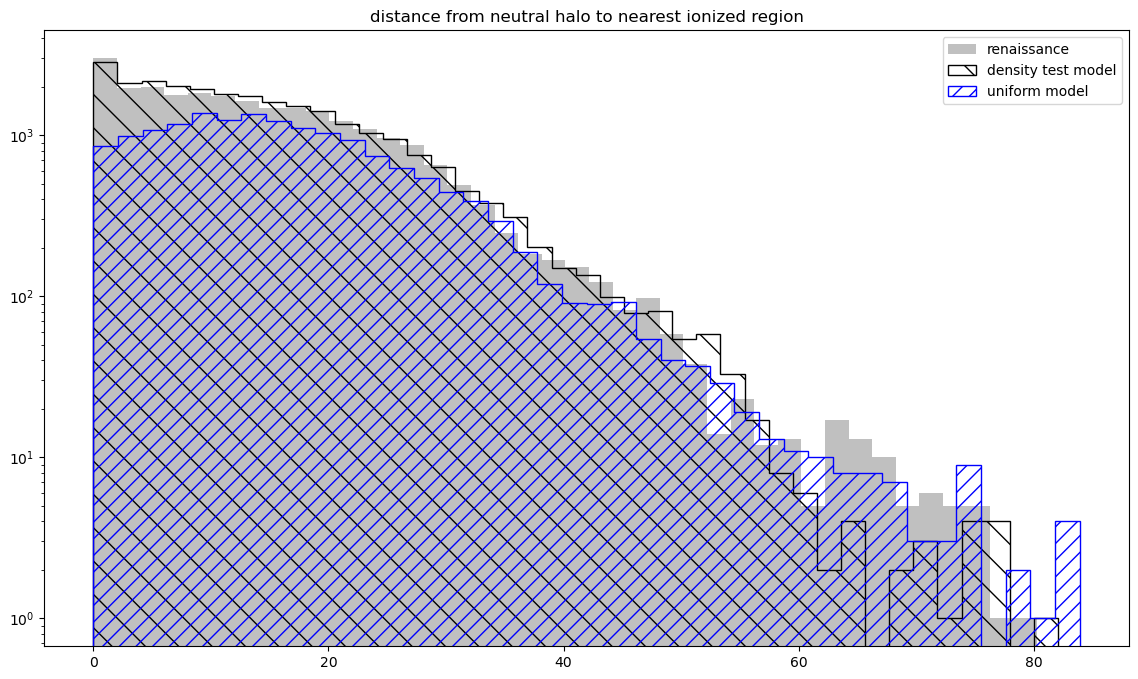 histogram showing the distribution of the distances to the ionized region for neutral halos.
These results didn’t show any particular difference between the sets, and as such I decided to refrain from further refinement on these plots for the time being.
Future Work
Before next meeting, I am planning on an additional change to the model that will hopefully resolve the scale-based geometry problems that I observed as a result of my most recent changes. In theory, instead of iterating over a set of different kernel sizes, I could instead create a single kernel that combined the effects of the other kernels; the photons would be spread out according to their distance from the source, and could be made to follow the distribution that would be caused by an infinite number of bubble scales.
My thinking is that, by doing this, I can eliminate the effects caused by the gaps between each bubble scale.