Research Update - Week 20

YSOLab

Zoomed-In Plots of YSOVAR Data

The Motivation

    As part of the larger set of Spitzer data we have, we have obtained data from the YSOVAR project, which consists of very high cadence observations of a small subset of sources. These observations were taken on the order of every few hours, usually for a month or so. This presents a small problem, as our usual data is on the cadence of every 6 months or so, so any larger variation in the YSOVAR b ecomes very suspicious when viewed from this zoomed out timescale.

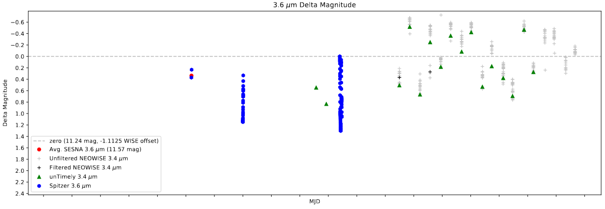A view of one of the curves where the YSOVAR data was particularly concerning.

    To address this, I quickly wrote an additional function within the script to generate an additional set of light curves, this time limited to just the YSOVAR data. The resulting light curves shed a lot of light on the subject, and generally made the behavior of the YSOVAR data much more ‘believable’.

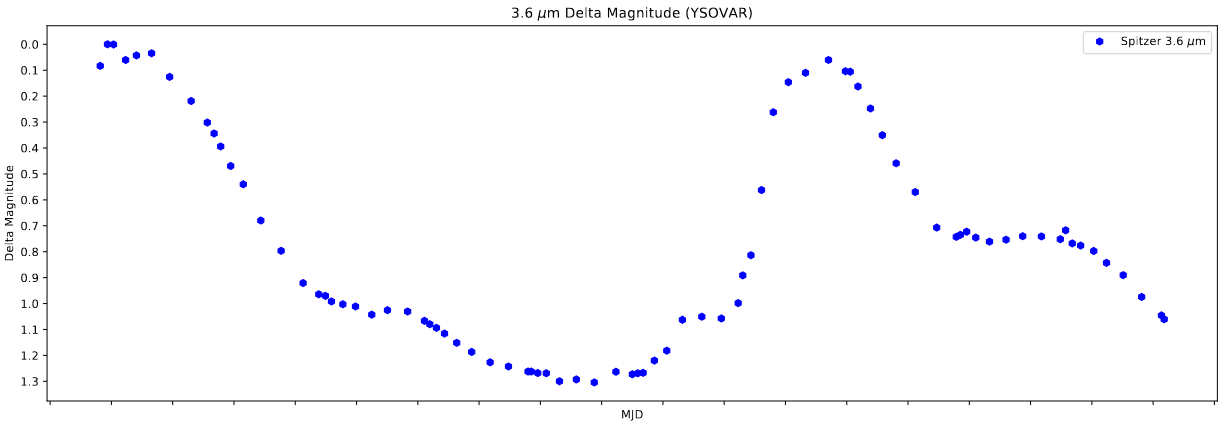The zoomed graph showing one of the two sections of YSOVAR from the above curve. This example is particularly interesting, and better explains the larger range seen.

Additional Wrinkles

    One additional wrinkle presented itself when I tried to use this light curve on every region in our set. What I noticed was that, for Rho Ophiuchus (and the other regions, on closer review), there was actually more than one set of YSOVAR data, usually separated by more than 100 days. This presents a problem, as the resulting timescale of plotting each of these sets together is much to large to properly display the minute variations between each point, as shown below.

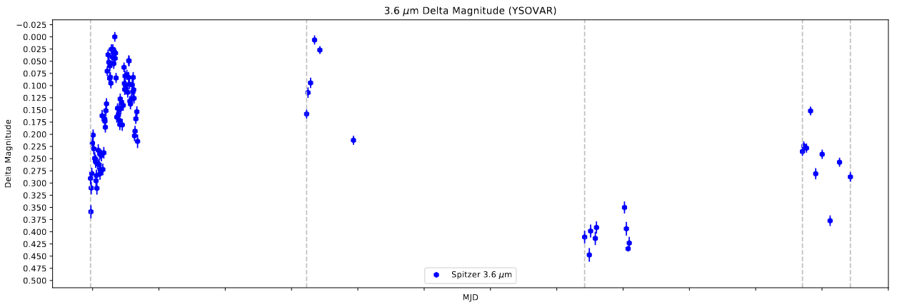A plot showing an graph containing all of the YSOVAR data for a specific source.

    To address this problem, I added some additional logic to my YSOVAR light curve generator. It first identifies where the gaps are using a difference calculation, then stores the index of the first point in each set. These indices are then iterated through, creating a set of multiple light curves, one for each of the YSOVAR sets.

    This does result in a number of less interesting light curves, but it does help better highlight the specifics of each YSOVAR set, which is as desired.

Future Work

    For next week, our plan is to start writing up each of the bursts we identified at our previous meeting. We have an overleaf document created, and the goal is to have each of the burst light curves added to the document, accompanied by a list of other names, and a brief summary of any previous literature on that object.

Gun Violence Archive Analysis

Clarifications on File Structure

    One thing I talked with Dr. Lilley about this week was the actual structure of the file. This helped to dispel several assumptions I had made regarding the structure of the files, and validated my choice to aggregate to the agency-year level.

    One other issue we identified is that there is likely some inconsistency with how the ‘months_reported’ column was used, which results in some agencies that did report a full year of data not accurately recording that fact.

Future Work

    With this new information, I should be able to have the aggregation code finished soon, and I can apply it to the other year files, as up until now I have been experimenting only with the 2017 file.

    I will need to address the months_reported issue, which should be possible using the months_included_in columns.

Cluster Research Pod

Meeting with Collaborator

    This week we met with our collaborator, who helped explain the process of centering to us. This presentation was an excellent resource, and helped validate and motivate some of the observations we had made during our own centering attempts.

    We also discussed our photometry code and its current issues, and we made plans to exchange the code, as well as some examples, so our collaborator could look over it, and offer any suggestions.

Identifying an Issue with Photometry

    While preparing the photometry code to send to our collaborator, I identified an issue that is likely one of the core outstanding problems with our photometric process.

    Sorry in advance if this section is a little strangely formatted; I am copying most of this text from an existing writeup I sent to the group.

Aside about Units

    One thing I verified during this process was the units of the existing images I have from JWST and from HST.

BUNIT = 'ELECTRONS/S' #HST
BUNIT = 'MJy/sr ' #JWST

    I am making the broad assumption that the PHANGS photometry, which is being done on HST images, is done with files with matching units. This caveat is important, but, as I will explain later, isn’t actually integral to my point, and my change is still defensible if this assumption is false.

Difference with Given Photometry

I was looking at the PHANGS photometry, and I noticed that the basic operations they use to get the photometry are as follows;

image = <load HST image>
image = image * counts

<aperture photometry on image>

flux_density = (aperture_sum - tot_bkg) / counts

<calculate magnitudes>

However, when I looked at our current photometry, I noticed that our process is slightly different;

image = <load HST image>
image = image #!!!

<aperture photometry on image>

flux_density = (aperture_sum - tot_bkg) / counts

<calculate magnitudes>

    My understanding, after looking at this, is that ‘counts’ acts as a unit conversion in the HST set, and is converting the counts per second to a different unit, which is then unconverted later. If this is true, then our current set, regardless of the units being correct or incorrect, is performing only half a unit conversion. If the original image units are the same between the PHANGS photometry and our photometry, then we need to multiply our image by counts.     If the original image units are different between the PHANGS photometry and our photometry, then we need to remove the existing dividing by counts from the flux density section. In either case, something about our photometry is faulty. This is purely my fault, as I didn’t really have a strong understanding (and still really don’t) of how the units of the image are being converted into magnitudes, and as such I could have easily ported one section incorrectly and not noticed.

Applied to SEDs

    To test this idea, I ran the photometry again, for both cases (removing [/ counts] and adding [* counts]). In both cases, the resulting SEDs were significantly closer to what I think we were expecting, as can be seen from the attached examples.

    They also happen to be visually identical in all cases, which does make some sense when you consider that both cases have the same net change on the numbers, and the aperture photometry section is operating in the same way regardless.

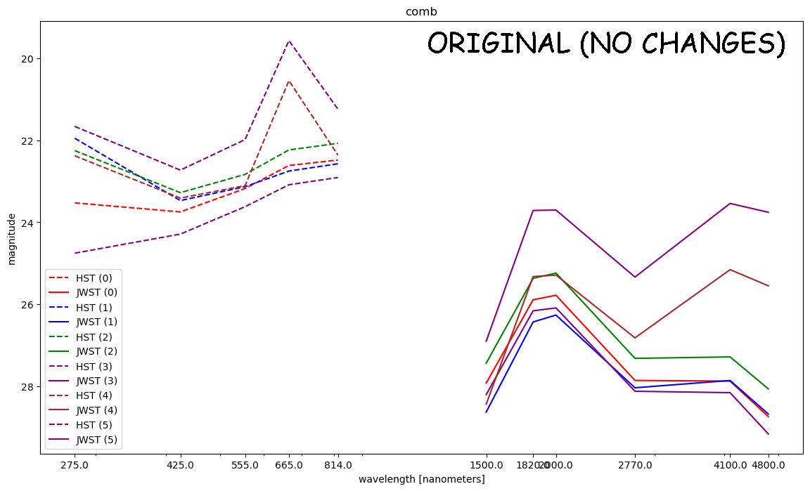A view of a set of SEDs for some sources, obtained using the original photometry function.

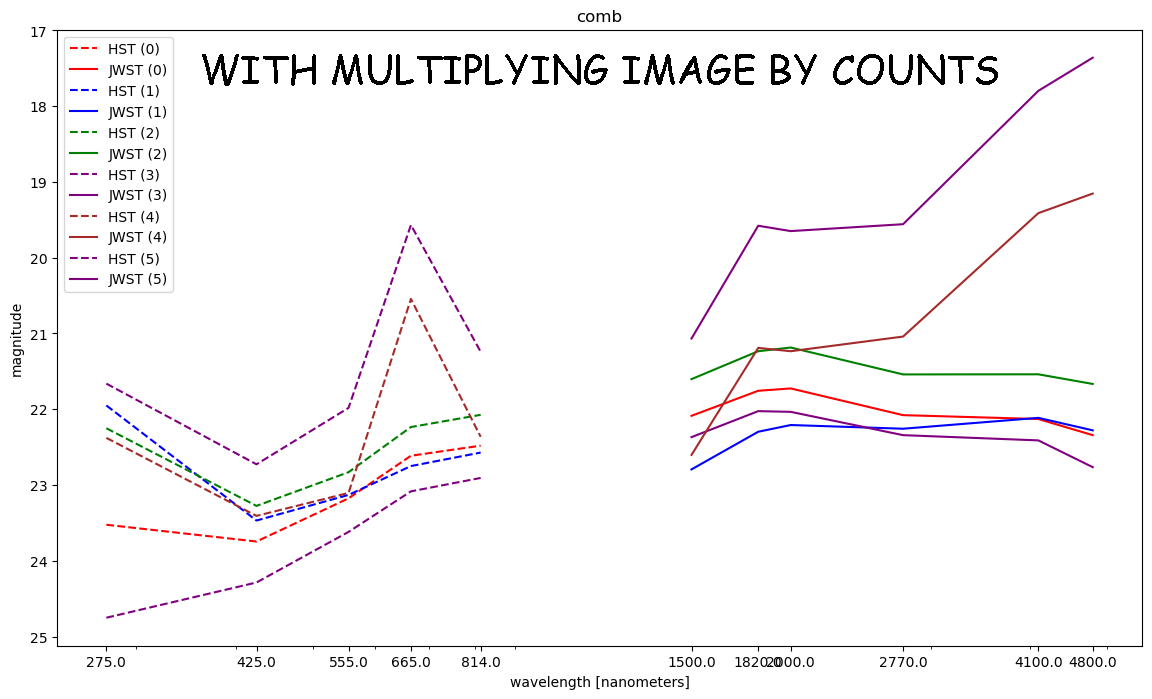A view of a set of SEDs for some sources, obtained using a modified version of the photometry that included an additional * counts.

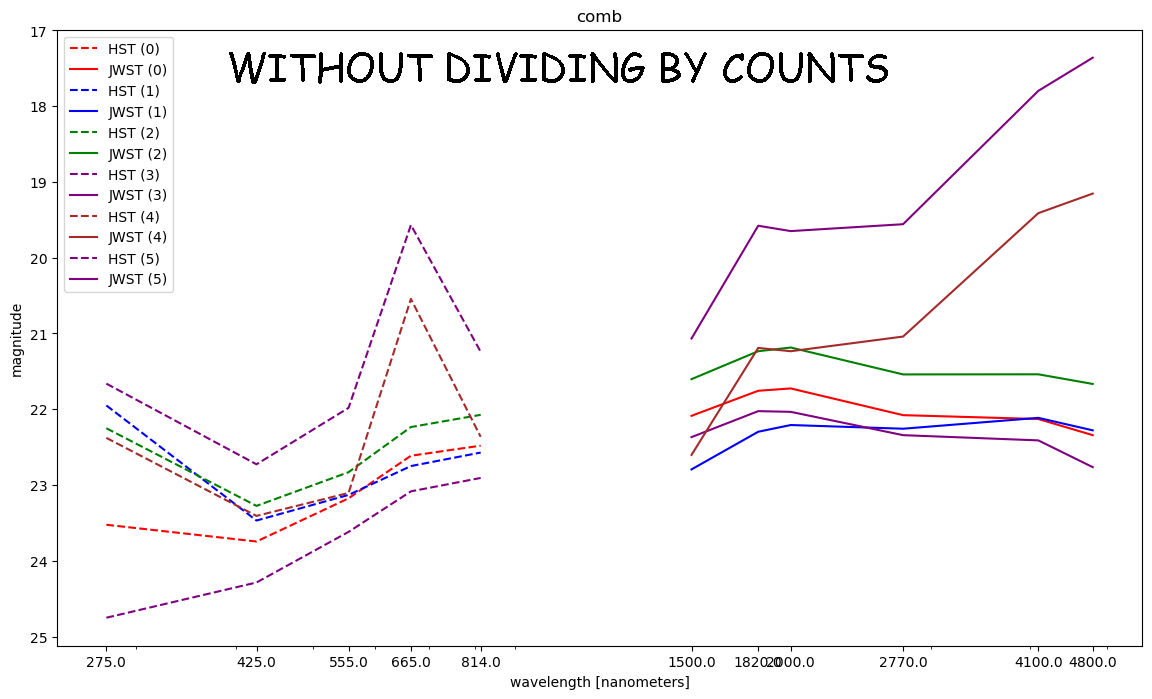A view of a set of SEDs for some sources, obtained using a modified version of the photometry that removed the mentioned / counts.

Remaining Questions

    One other wrinkle in this change is the difference in how the variable ‘counts’ is being calculated between PHANGS and our method.

counts=header['EXPTIME']/header['CCDGAIN'] #PHANGS (HST?)
counts = topheader['EFFINTTM'] / header['PHOTMJSR'] #Our method (JWST)

    Another outstanding assumption is that the given ModifiedPHANGSPhotometry file is meant for HST images, and not a modified version meant for JWST images. This is supported by the header names used, which do not appear in the JWST images. However, if this assumption is incorrect, I don’t think it impacts the overall claim too strongly, as it would just mean that we are meant to match the methods within, which I have shown to be functionally equivalent to removing the extra division.

Future Work

    My immediate next goal is to dig into the photometry function and write out the units of each of the input values, then trace those units through the function to verify what each of the values is doing, and what conversions we should or shouldn’t be performing.

    I also still need to package up and prepare the photometry code to send to our collaborator. This has been put off slightly by the recent discovery, and I want to make sure that I have addressed this outstanding issue before we send the file.