Research Update - Week 6
YSOLab
Future Work
For next week, each member of the group was assigned a portion of the sources in the Ophiuchus to manually verify. This involves checking the outputted fits table data for any oddities, checking the SESNA image of that source to verify that the source isn’t a binary, or is being affected by some nearby objects.
One thought I had was that instead of using a program like DS9 to manually find each source in the very large SESNA image, I could instead write a small script to generate a thumbnail image of each source from that image. This has the benefit that I could generate all of these, and compare them against each other very quickly.
Cosmology Group
Identifying Filaments with Clustering Algorithms
Several of the improvement avenues we identified from our brainstorming rely on being able to identify the location of filaments within our simulation box.
Mihir, a post-doc working with us, mentioned that previous papers had made use of a Friends-of-Friends algorithm to identify halo positions from a density field, but that they also inadvertently identified what appears to be filaments at the same time.
I made use of the scikit-learn package to implement several different clustering algorithms in my attempt to replicate these previous results using the overdensity cube of dark matter we have been working with.
These algorithms are more addressed towards a list of points, rather than a continuous cube input. To match this, I wrote a small script that selected points above a certain threshold in the density cube, then extracted the positions of those points into an array, which could be fed into these algorithms.
Agglomerative Clustering (Friends-of-Friends Adjacent)
My initial attempts were focused on the Agglomerative Clustering algorithm, as I had found online that it functioned equivalently to a Friends-of-Friends algorithm.
The first hurdle I encountered was in trying to run this algorithm on a very large set of points. The algorithm itself was only able to take an array of point positions directly if the points were in 2D space, but it was also able to take in a distance matrix, which contained the distances from each point to every other point. The problem becomes that, since there were more than 50,000 points, the resulting distance matrix would have taken up nearly 200 GB of memory.
To get around this, I leveraged a few things. I increased the density threshold, which reduced the number of points to about 20,000. I also forced the matrix to use 8-bit integers, as opposed to 64bit floats. These changes brought the memory requirements down to about 500 MB, which is much more manageable.
Unfortunately, the results of this were less than spectacular, and did not really effectively isolate the filamentary regions. This is likely due to the concessions I made previously, and could be improved with more careful consideration of the input parameters.
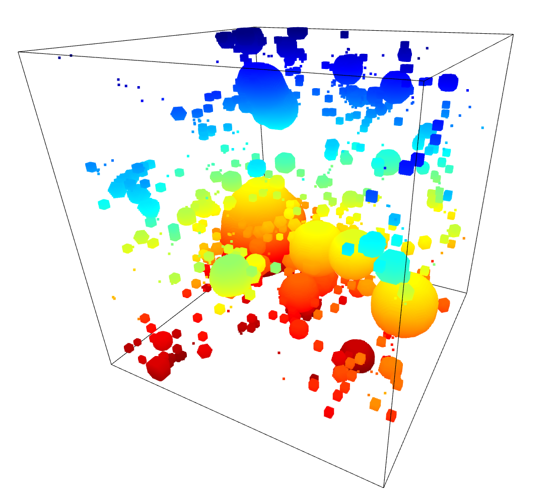
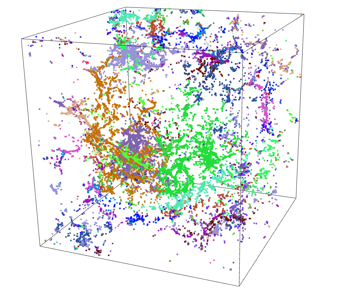 Results of Agglomerative Clustering (Clusters share a color)
DBSCAN & HDBSCAN
After the less than stellar success of Agglomerative Clustering, I decided to give a separate set of algorithms a try, specifically DBSCAN and the related HDBSCAN.
The benefit of these algorithms is that they are not limited to 2 dimensions, and as such can directly receive the array of point positions.
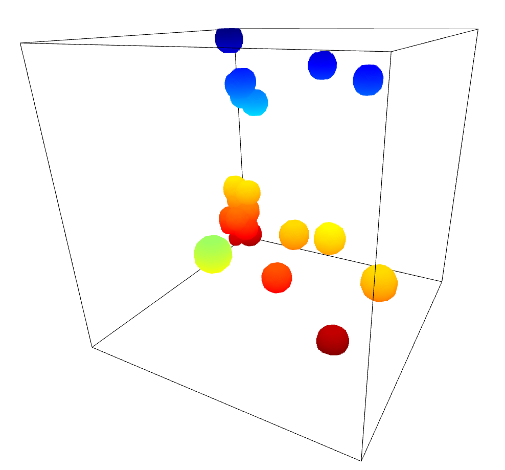
After some tweaking of the input parameters, and filtering out points that were not attached to a cluster, I recieved results that were actually very promising.
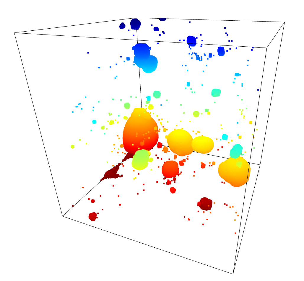
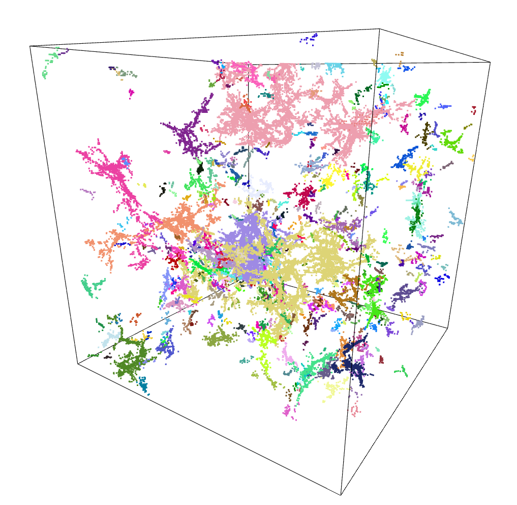 Results of DBSCAN (Clusters share a color) Results of DBSCAN (Clusters share a color) | 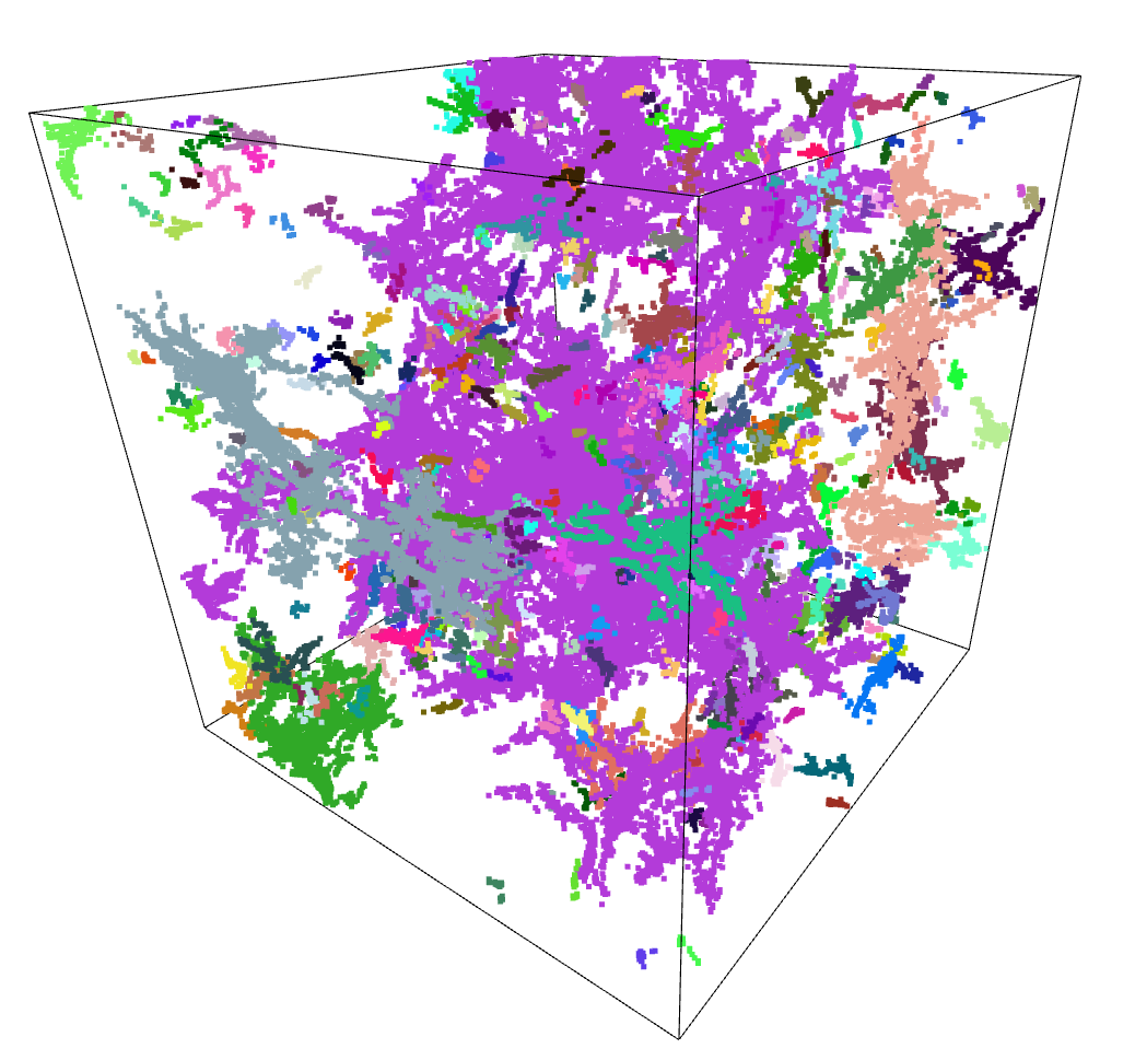 Results of HDBSCAN (Clusters share a color) Results of HDBSCAN (Clusters share a color) |
To test these results, I moved forwards using the HDBSCAN results. I subtracted away the pixels identified as part of a filament from the density cube, setting them to the average density inside the overall density cube. A quick comparison of the untouched density cube and the newly subtracted cube was less promising, as they showed very little change.
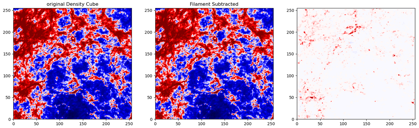 Results of Filament Subtraction (Final plot shows differences)
I confirmed this by running the model with this altered density cube. The overall results were essentially unchanged, with no noticable difference between the model when run on the unaltered density cube and the model run on the filament subtracted cube.
 Results of Model with unmodified density Results of Model with unmodified density | 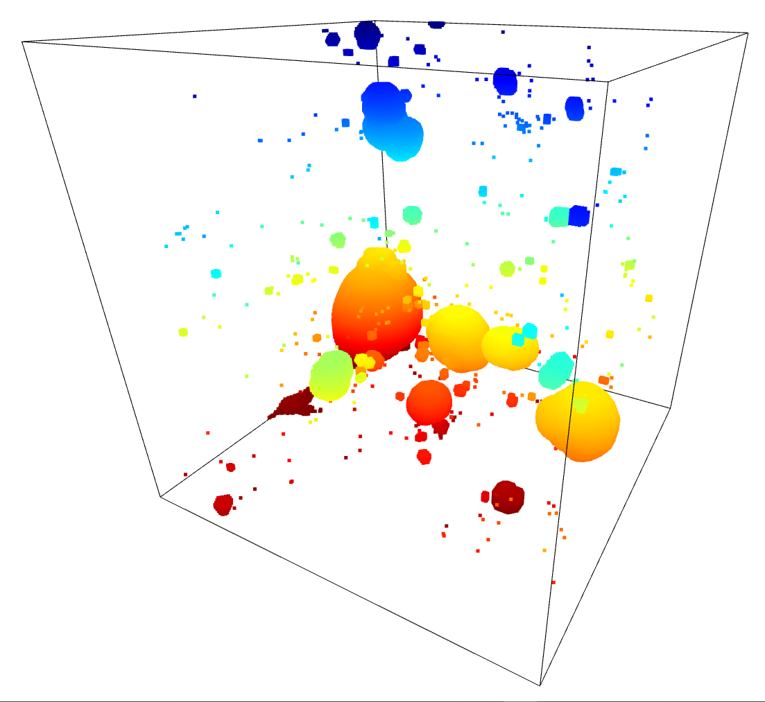 Results of Model with filament subtracted density Results of Model with filament subtracted density |
Varying Photon Threshold with Bubble Size
One other avenue to explore was to vary the photon threshold with the placed bubble size. This would allow us to correct for the effects of the pixel resolution on the resulting bubble.
For the majority of bubbles our model overshoots the intended bubble volume by 8x for isolated bubbles, and by 4x for unisolated bubbles. Previously, we had implemented a flat 1/4 multiplier to the number of photons in order to correct for this effect. However, some testing revealed that the effects of the pixel resolution meant small bubbles would overshoot the volume by less and less, down to no overshooting for bubbles with a radius of 1.
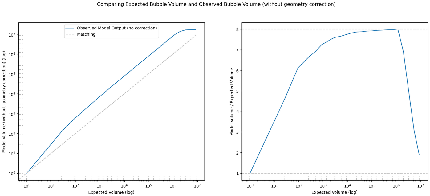 Plot of the bubble volume overshooting on an isolated bubble
To solve this, I wrote a small function to approximate the needed multiplier to counteract the overshooting from the selected bubble size.
\[y\ =\ e^{\left(-1.25\left(x-.15\right)\ +\frac{3}{4}\right)}+\frac{1}{4}\]I them modified the model code to apply the multiplier during the bubble placement portion. I then compared the model output using this change to one where I gave it a set of all 1/4.
Overall, the results were less dramatic than I might have expected. However, in hindsight, only the very smallest bubbles would have been measurably affected by this change, and even then the actual effect is likely fairly minimal.
 Results of Model with constant 1/4 threshold Results of Model with constant 1/4 threshold | 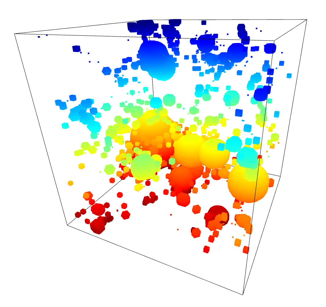 Results of Model with bubble size dependent threshold Results of Model with bubble size dependent threshold |
One additional test I did was to set the multiplier to 0 for all bubble sizes except for one, in order to verify that the model changes were working as expected. The results were as I expected; only a specific size of bubble was placed.
 Results of Model with constant 0 multiplier except for a single bubble size
Future Work
For this next week, my goal is to implement the halo slice plots from before on the model and density outputs of these two new methods. Those plots would allow us to more clearly observe any smaller-scale changes in the model outputs or density cubes.
I will also try working on the filament finding process some more. This could include trying a different clustering algorithm, such as Spectral Clustering or OPTICS, as well as a method for ‘expanding’ our filament selections to include a radius around them, in order to capture more of the density field than just a thin tube through the center, perhaps replacing these regions with a larger radius smoothed density, rather than 0?
Gun Violence Archive Analysis
Comparing City-Level Data with Other Sets
The majority of my work this week was again focused on looking at a few major cities, this time in comparing the results from several different datasets to the GVA results. Specifically, we wanted to compare the gun-based homicides found in the FBI Homicide dataset and the CDC Mortality dataset with the GVA deaths over the same period.
The FBI Homicide dataset was fairly straightforward to implement, as I already had most of the machinery in place, however the CDC data took some more doing than previously. I was able to leverage the CDC WONDER page to selected and download a count of deaths caused by ‘Assault by firearm’ by county and year.
I then plotted this data by selecting for 4 specific cities of a decent size; Atlanta, GA, Baltimore, MD, Chicago, IL, and Cincinnati, OH.
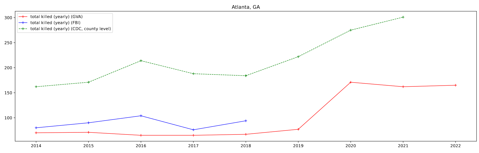 Plot of Data for Atlanta, GA
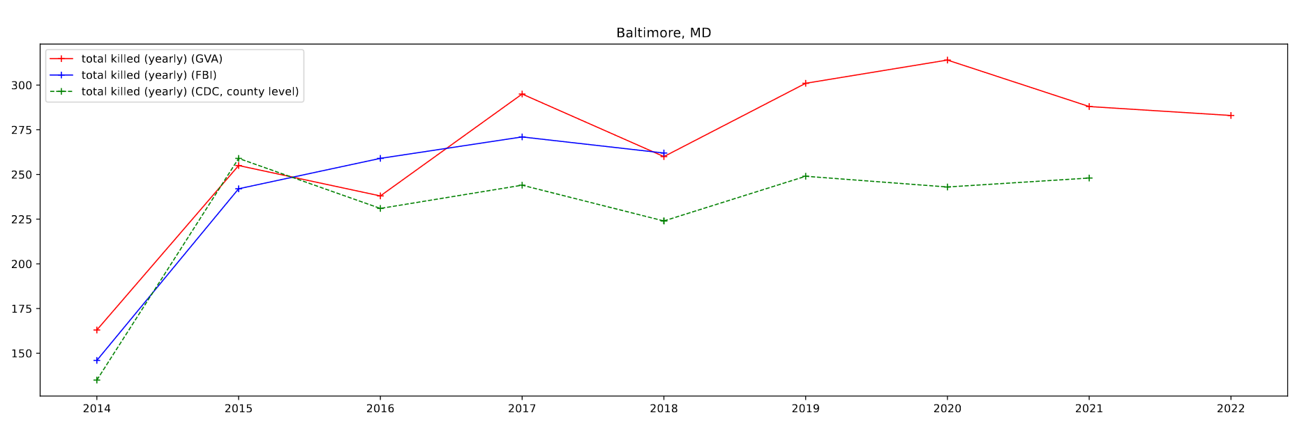 Plot of Data for Baltimore, MD
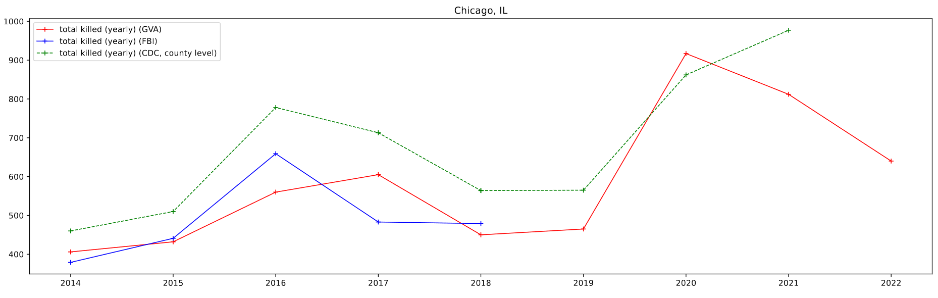 Plot of Data for Chicago, IL
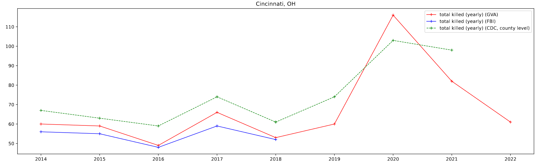 Plot of Data for Cincinnati, OH
One foible that can be seen is the CDC data, which doesn’t follow the other data as well. This can be partially attributed to the lack of place fips codes available for the CDC data. As a result, I am selecting by county, which in most cases is a differently sized area to the place designations. For Atlanta, which lies in between two larger counties, the results are particularly pronounced.
Future Work
One area of work for next week is to compare the CDC data I have downloaded with a set of pre-existing data that Dr. Lilley has collected that covers 1990-2016, in order to verify that these counts match.
I will also try to integrate the data shown on the AFPI report that sparked much of this work, in order for easier comparison.
One other point of interest is an odd quirk that Dr. Lilley has noticed when he has worked with CDC data previously. Specifically, he has noticed that, for privacy reasons, counties with more than 0 but less than 10 deaths in a year are not included in the set. I plan to check the counts in the set to see if this behavior is present.
Galaxy Cluster Pod
Creating Preliminary Training Set
Part of our tasks this week was to start putting together a training set of clusters from our existing cluster catalog.
Of particular interest were clusters that were particularly bright in H-alpha, and clusters that were brighter in I and V, and faint in H-alpha, indicating older clusers.
Using the Sundog viewer and a script to identify clusters from pixel positions, I put together a set of clusters for both criteria. Both the Color-color diagram and the SED for these clusters seem to match what I expected from them, which is a good verification of what I found.
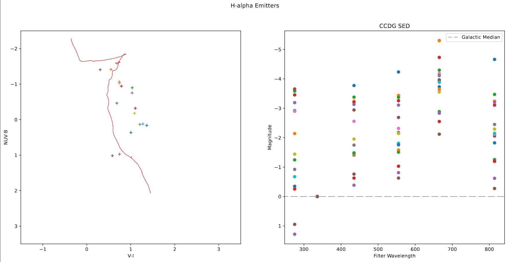 CC Diagram and SED for H-alpha emitting clusters
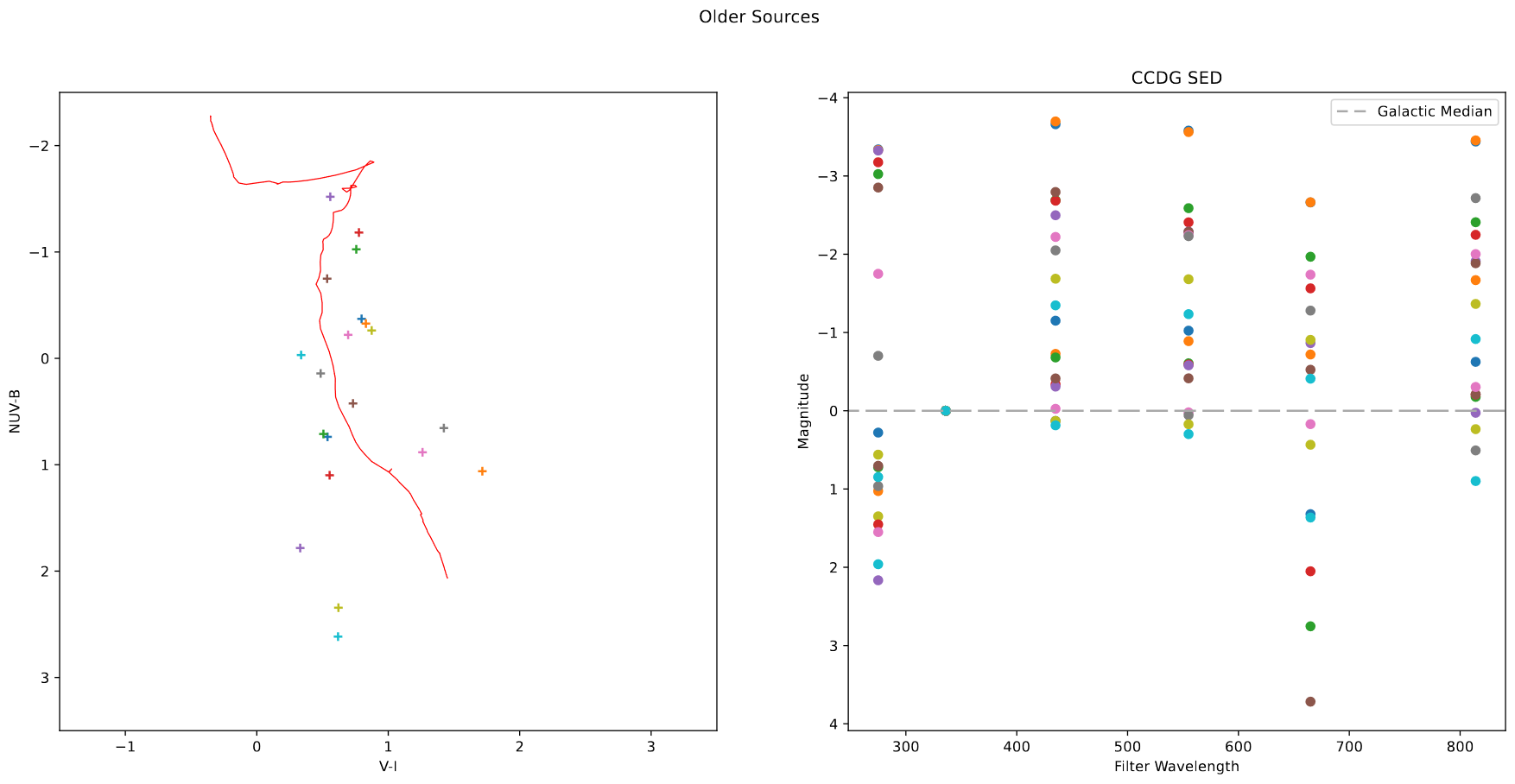 CC Diagram and SED for older clusters
 Plot of chosen H-alpha emitting cluster positions Plot of chosen H-alpha emitting cluster positions |  Plot of chosen older cluster positions Plot of chosen older cluster positions |
In the end, we decided to focus first on extracting a new cluster set from our newly recieved JWST data first, so these sets will be placed on the shelf for the time being.
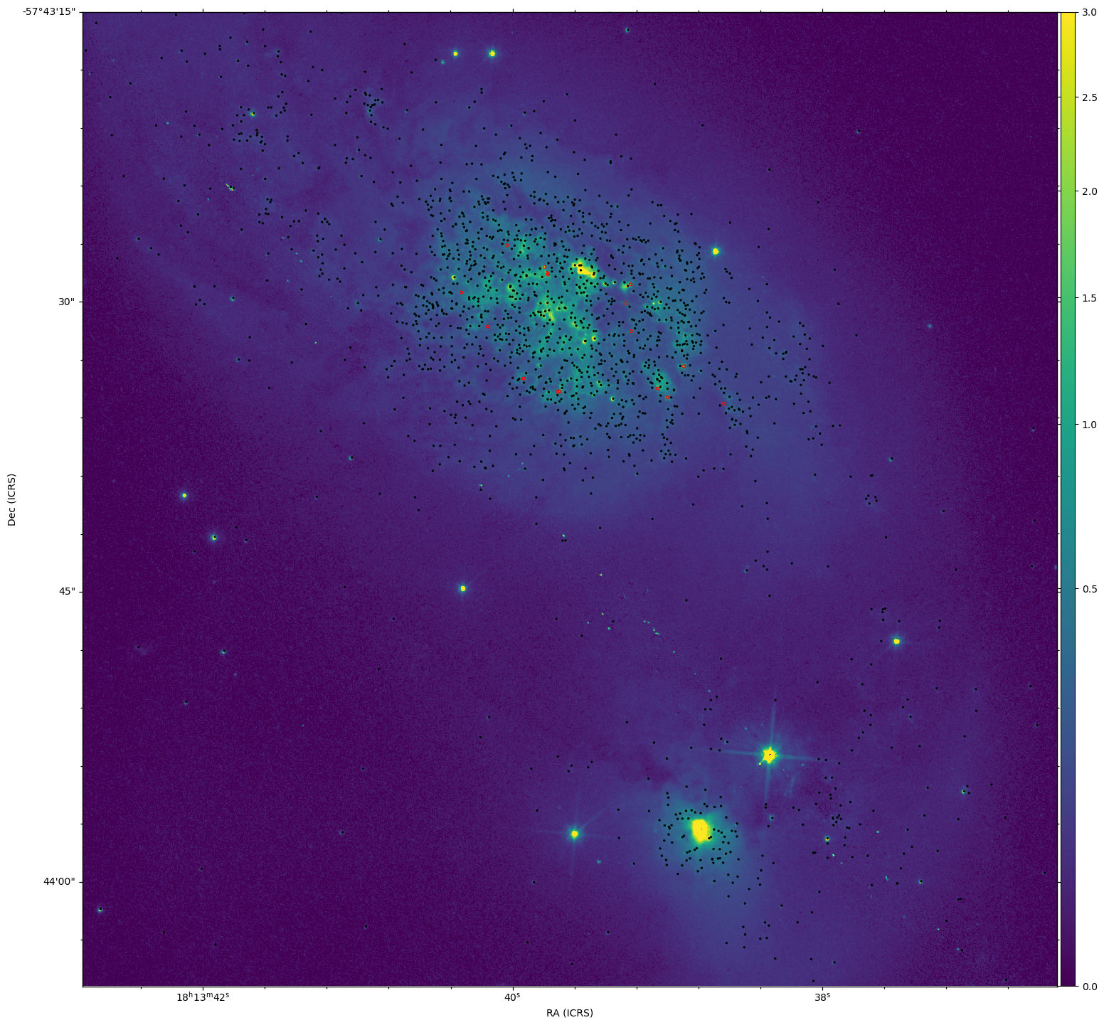
Approaching Photometry Problems
Our main assignment for next week is to experiment with the star-finding algorithms to identify clusters within the JWST images we have recieved. Our method revolves around the DAOStarFinder and IRAFStarFinder from the photutils package, with which we use the parameters FWHM and threshold, which is some multiple of the standard deviation.
In order to get some sense of how these variables change the results, I selected a grid of possible FWHM and threshold values, and ran the two starfinding algorithms with this grid of points on the same image, and counted the number of objects identified.
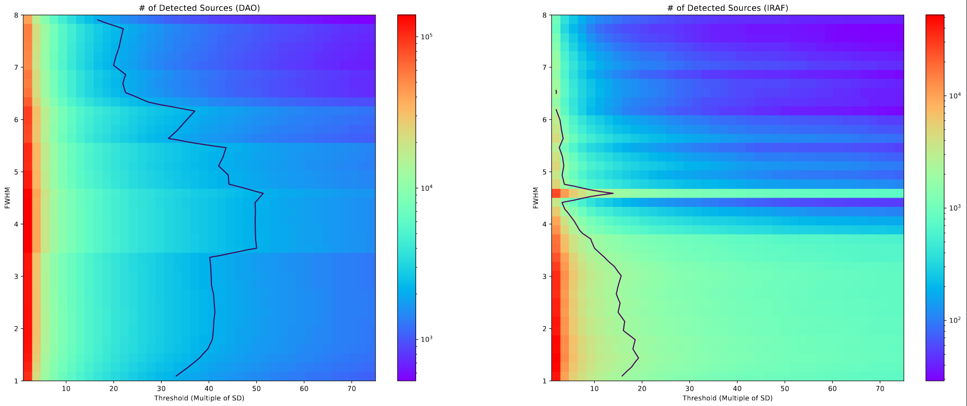 plots of the number of clusters found for a grid of FWHM and threshold values
I also plotted a contour line showing the number of clusters in our previous cluster catalog for this object. The inclusion of this line is somewhat sketchy, as there is some amount of interpolation being performed by matplotlib during the plotting process, however the overall shape is still useful.
Our output from this process needs to have more found objects than the number of clusters in the old catalog, as we expect to find more clusters in this more accurate and less extincted JWST image, and there are several additional filtering steps we still have to perform before we land on a final set.
Therefore, the set of usable FWHM and threshold values will lie somewhere to the left of the contour line showing the old cluster count.
Future Work
As mentioned previously, the main goal for the next week is to experiment with the star-finding algorithms, and try to get some sense of their behavior before we pick one and narrow down the best FWHM and threshold values.