Research Update - Week 9

YSOLab

Examining Variability

    Our main goal over the last two weeks has been to work through our group of sources and identify, by-eye, the general behavior of each object by classifying as Fade, Burst, Fluctuations, etc.

    After doing this for my set of sources, we spent our meeting time working through the more interestingly designated sources, and confirming our selections. We were able to do this for a number of sources, however due to time constraints we couldn’t address every source.

Future Work

    The main thing I will br working on for next week is a set of plots related to the color of each source in our list. During our discussion of the variability designations, we noticed a number of sources with both subtle and significant disconnects between the two wavelength bands we are examining. To visualize these differences more clearly, Dr. Megeath suggested that we use a two plots, with the common thread being the color of the source, which was just the magnitude in one band minus the magnitude in another. Specifically, visualizing the color over time, as well as the color vs the magnitude, would help us better characterize the behavior of the source’s color, and pick out instances of uncharacteristic behavior.

    One other plot will work on for next week is one that compares the different scales of variability. From what I understand, this plot is constructed by comparing the magnitude difference from each point to every other point with the timestep difference between each of these points. The goal of this would be to see at what timescales the majority of the variability is happening.

Cosmology Group

Fixing Mistakes in Recombination

    The first thing I tackled this week was fixing some of the initial mistakes I had made in my implementation of recombination into the semi-analytic model. The first of these mistakes was in my mixing of comoving centimeters (in the gas density and the pixel volume) and proper centimeters (in the constant used for calculating recombinations. This was fairly simple to fix by bringing in the redshift and converting from comoving centimeters to proper centimeters.

    The next mistake to fix was in my failure to consider the recombinations cumulatively; in my previous implementation, the number of recombinations since the last timestep was being compared against the total lifetime photons in each pixel. This was another fairly simple fix, where I just carried, between each step, a cube containing the total lifetime count of recombinations in each pixel, and added the new timestep’s recombinations to that cube.

Implementing Halo-Based Recombination

    The next major thing I worked on this week was to implement a variant of the recombination method that Dr. Visbal suggested during our previous research meeting, where instead of subtracting the recombination counts from each pixel, I would associate the recombinations in each pixel with the responsible halo, and subtract photons from the halo directly.

    Given my further goals and time constraints, I decided to implement a slightly simplified version of this method (as suggested by Dr. Visbal), where instead of trying to specifically associate each pixel with the (likely several) halos responsible for its ionization, I would instead gather all the recombinations in that timestep together into one total count of recombinations, then divide them out to each halo based on its fraction of the total stellar mass, so that halos with more stellar mass would get more recombinations. Our understanding was that this method would be a very decent approximation, and would allow us to move forward with testing and refinement.

    I was able to implement this using much of the same code from the original implementation, except with an additional step where the recombinations in each pixel are collected and redistributed to each pixel based on stellar mass; since only pixels that contain halos would contain stellar mass, this has the intended effect of associating the recombinations with halos based on stellar mass, without needing to specifically associate each halo with a recombination count.

Initial Results of Modifications

    Following these changes, I ran the semi-analytic model with both the space-based and halo-based methods, and collected some more specific results in order to better understand the behavior of the model.

    The output of these tests was very illuminating, in that they showed that the current implementation is wildly wrong in some fundamental way. Specifically, I kept track of the total lifetime number of recombinations and photons in the model at each timestep, then graphed these counts, as shown below.

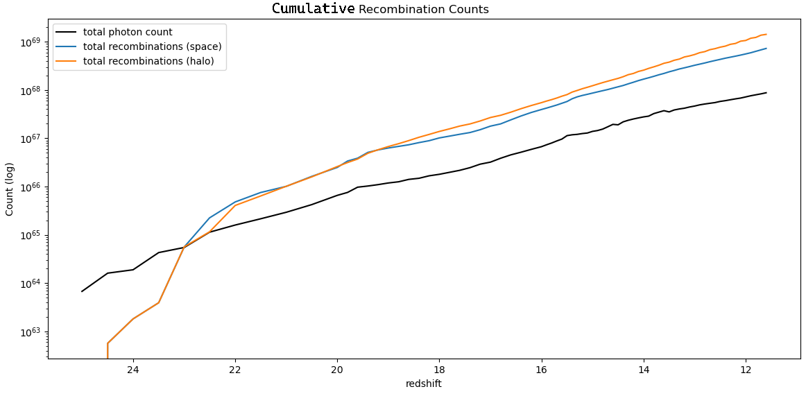Plot showing the cumulative number of photons and recombinations in a semi-analytic model run

    The clear problem is that, past a certain point, there are more recombinations in the overall box then there are photons, which shouldn’t be physically possible.

    After consulting with Ryan and Mihir, understanding and explaining this behavior became my primary focus for the rest of the week.

Simplified Recombination Testing

    To try and better explain the wildly incorrect results of the current model, I pursued instead a very simplified case, where we had a single halo with a set mass in the center of an otherwise empty simulation box.

    I could then calculate the number of photons the halo would produce, and the number of recombinations that would occur over a certain length of timestep.

    This testing produced results that were consistent with the model; placing the same setup within the model results in an equivalent count of photons and recombinations.

    One interesting note from this process is the length of each timestep within the renaissance simulations. Specifically, the timesteps are not of equivalent length.

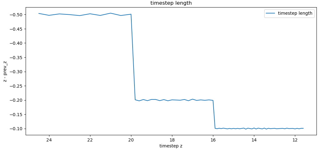Plot showing delta z from the previous timestep at each timestep

Further Significant Mistakes in Recombination

    While communicating the results of my recombination testing with the group, we came across two significant mistakes in my implementation that were likely the primary result for the disconnect between the photon and recombination counts.

    The first of these mistakes was in converting from comoving to proper centimeters. I had messed up that relation, and had inverted the fraction so that instead of dividing by 1+z, I was multiplying by 1+z. This was a relatively simple fix to implement into the simplified calculations, and helped correct the redshift dependence that was displayed.

    The second and much more significant mistake was in my calculation of the timestep length. While implementing, I had relied on some code take from earlier in the model, which had been labeled as calculating the timestep length in hubble time, which I found a conversion to seconds for online. I took and reused this uncritically, which is where I had made my mistake. In reality, the calculation I was performing was returning the timestep length in years, rather than hubble time. This resulted in a timestep length that was nearly 10 orders of magnitude higher than would be correct, and is likely responsible for the majority of the disconnect.

    After quickly fixing these issues in the simplified calculation, we get a number of recombinations that is significantly closer to our expectation, as evidence by the below plot.

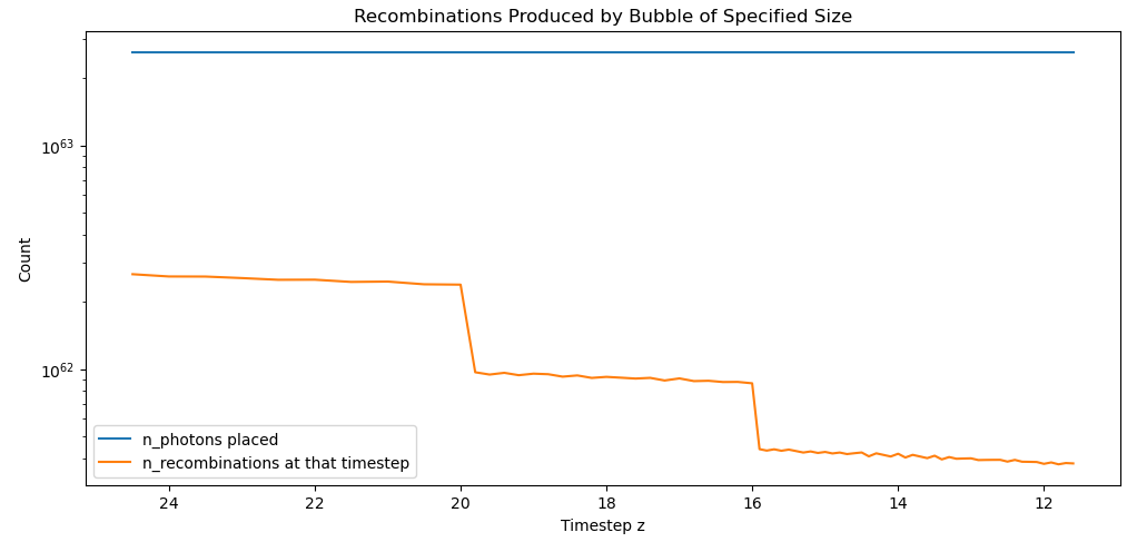Plot showing the number of photons and recombinations calculated for a specific timestep

One thing to note is the steep drop in recombinations made past a certain timestep; this is almost certaintly due to the change in timestep length, as the timestep lengths become much shorter at those redshifts, resulting in fewer recombinations being produced in each timestep.

Future Work

    For next week, my first goal is to correct the previously elaborated mistakes within the model itself, and observe how this affects the model output, with the hope that we will observe much more physically accurate output than previously seen.

    I will also work on constructing the ODE for the recombination rate over time; currently, we assume that the recombination rate is constant throughout the timestep, when in reality as the ionized regions recombine and the halos emit photons the recombination rate will change. Our plan is to construct the ODE representing this process, then solve it such that we can account for this effect in the recombination count.

Gun Violence Archive Research

Graphing Dataset Difference

    My primary work this week was in trying to graph the differences in the GVA, FBI, and CDC sets of gun violence deaths organized by county and year vs both the year, as well as the population.

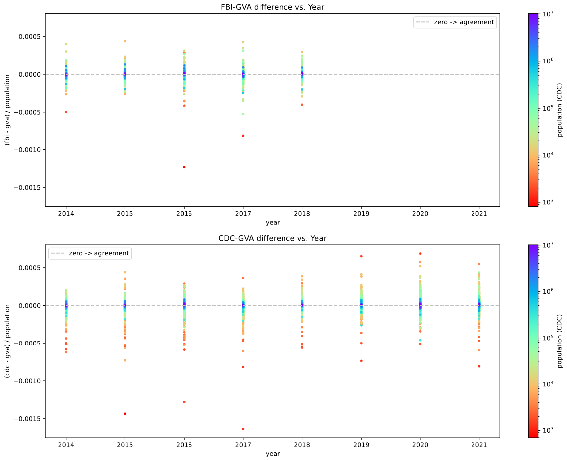Plot showing the difference between the GVA and FBI counts (divided by the population of that county) vs the year

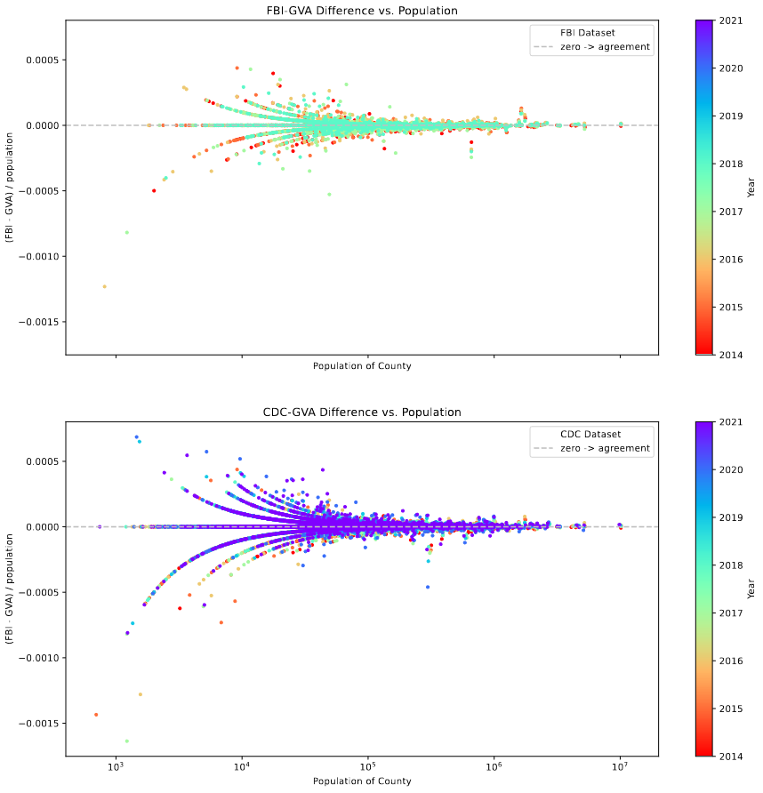Plot showing the difference between the GVA and FBI counts (divided by the population of that county) vs the population of each county. The odd shape is likely a result of the dependence on population in the y-axis.

    The main result of this is some significant evidence of ‘heteroskedasticity’, where the error in our variables changes based on other variables, in this case population. We can see this from how the redder points in the first graph, which represent areas of lower population, tend to have larger error, while the higher population counties have less error.

    This matches with Dr. Lilley’s expectations, as his experience is that, in general, smaller population counties tend to have much larger error in most statistical datasets.

Future Work

    For next week, my plan is to work on implementing a number of basic statistical tests to compare the three sets. Specifically, using a t-test, ANOVA test, and a regression, with the goal of getting a better understanding of the differences between these sets, and to investigate whether the difference is dependent upon the year.

Cluster Research Pod

Mosiac Starfinding

    Our main goal this week was to develop a way of separating our image into many discrete sections, then run the starfinding algorithm on each of those sections individually, using that sections standard deviation to determine the threshold at some constant sigma value.

    I was able to develop the system as described, however the overall result was, in many ways, worse than what we had achieved with the starfinder on the entire image.

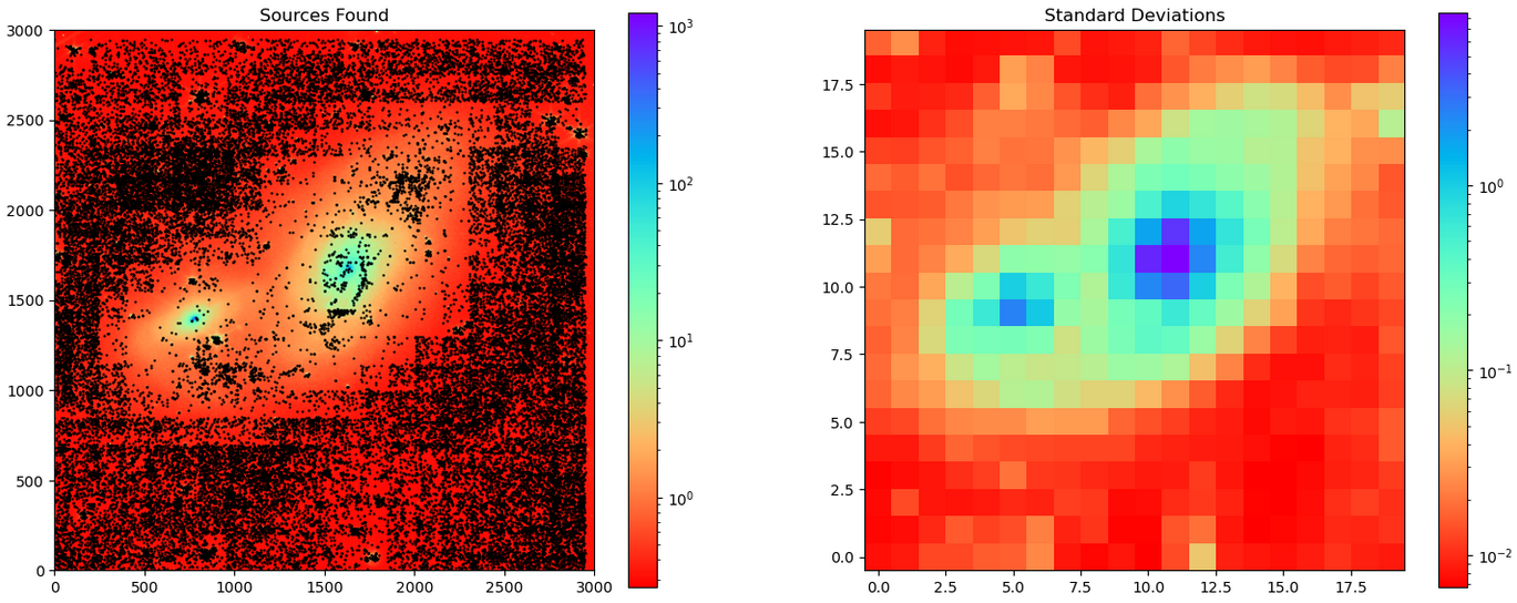plot showing the results of the mosaic starfinding on 200 pixel boxes with 100 pixel overlap. 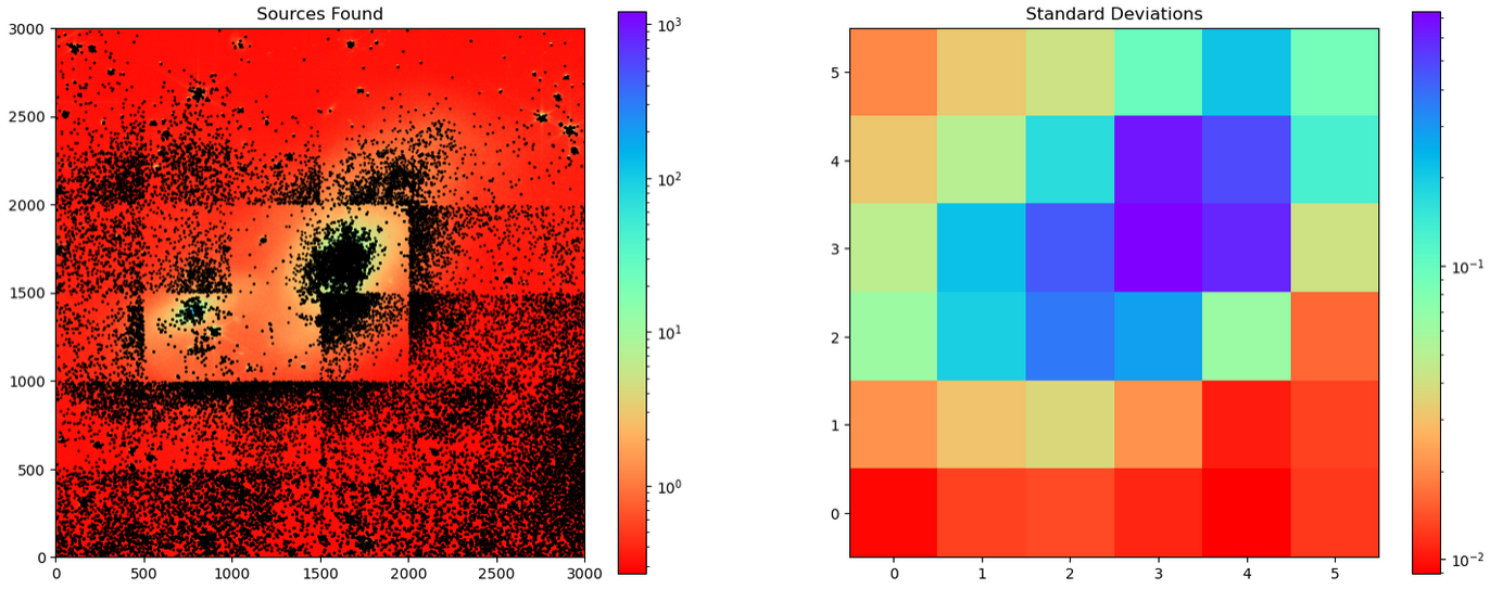plot showing the results of the mosaic starfinding on 1000 pixel boxes with 500 pixel overlap.

    In all cases, we see a number of artifacts and issues related to the edges of the boxes, where the edge of the box is clearly visible from just the different cluster candidates found, and in general clusters are only found in regions outside of the galaxy proper, where the standard deviations are much smaller, and therefore the threshold is very low.

    Several other members of the group were able to develop the same system in parallel, and their results matched mine, with many similar artifacts and general problems.

Future Work

    For next week, our goal is to try and find a method to increase the accuracy of our starfinder, with a focus on pre-processing methods, such as median subtraction, or a further refinement of the mosaic method.